I was recently asked to help with Comprehensive Future’s Fair Admissions Advisor. This provides general guidance on what effect different admissions policies have on school inclusivity. It also specifically reports on the socioeconomic profile of any secondary school compared to its surrounding area. Large Language Models are notorious for casually inventing ‘facts’ then confidently and articulately presenting these as the truth. My task was to ensure the data behind the Admissions Advisor provided an objective way to compare individual schools to the surrounding local area based on factual evidence.
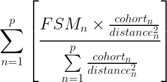
The initial ask was to match each of England’s 3,000 odd secondary schools to its nearest primary school and extract the proportion of children receiving Free School Meals (FSM) at each. FSM is commonly used as a proxy for socio-economic profile of school cohorts. However, just looking at the single nearest primary school would inevitably lead to some odd results. Based on some ideas I had from 2019, I suggested we look at several nearby primary schools weighted according to their cohort size and the square of their distance. This gives a simple model for the relative ‘influence’ of each neighbouring primary school:

The reason ‘influence’ diminishes by the square of distance is because, even if it isn’t formally defined, the effective catchment area of a school increases by the square of its radius. This is known as an inverse square law. It crops up wherever the ‘intensity’ of something spreads out over distance such as gravity, sound propagation, or even the wave energy from a stone dropped in a pond.
How it works
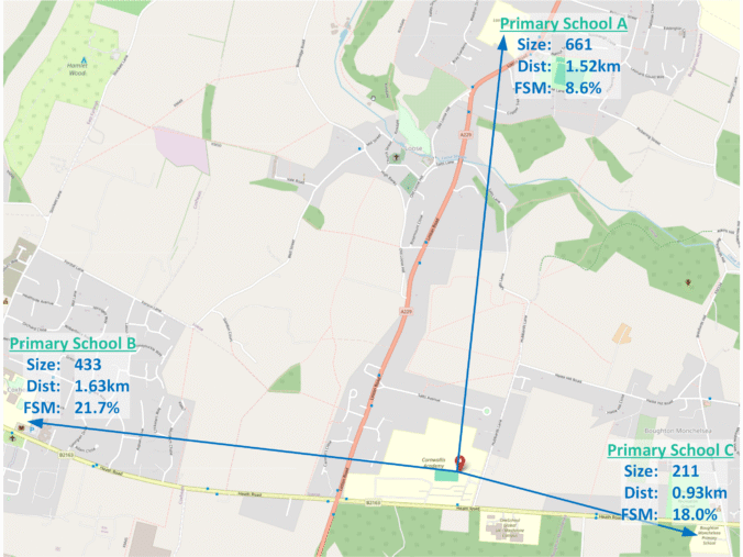
Here’s a simple example. It’s based on real data but, to keep it simple, only looks at the three nearest primary schools shown on the map at the top of the article. The first step is to obtain the Size – ie number of pupils, %FSM, and Distance for the primary schools nearest to the secondary school we’re looking at. These values are shown in the first three rows of this table.
| School A | School B | School C | (row sums) | ||
|---|---|---|---|---|---|
| #1 | Size | 661 | 433 | 211 | |
| #2 | FSM | 8.60% | 21.70% | 18.00% | |
| #3 | Dist(km) | 1.521 | 1.628 | 0.931 | |
| #4 | Size/dist^2 | 285.72 | 163.37 | 243.44 | 692.53 |
| #5 | weight | 41.26% | 23.59% | 35.15% | 100.00% |
| #6 | wght×FSM | 3.55% | 5.12% | 6.33% | 14.99% |
The remaining rows show how the final ‘local area’ FSM rate is calculated:
- #4: This row works out the relative weighting for each primary school based on its size divided the square of distance (
 ). These relative values can’t be used directly so the first step is to add them up (692).
- #5 This row takes each individual weight from row #4 and divides it by the total from the row above (692). The individual weights in this row now add up to 100%. In this example, roughly 40% of the weight goes to School A, 25% to B and 35% to C.
- #6 The final step is to take each weight from row 5 and multiply by the primary school’s individual %FSM from row 2. These values are then added to provide the overall ‘local area %FSM’ of 14.99%.
Although primary school C is the closest, A is over three times bigger, so its weighting is the highest. Primary A also has the lowest rates of FSM by a large margin. This brings down the final ‘local area’ FSM to just under 15%. A simple (unweighted) average would put too much emphasis on B & C’s higher FSM figures.
This example also demonstrates the problem of not checking enough local primary schools. Getting this right involves some ‘tuning’. The final version checks the 18 nearest primaries and ‘local FSM’ for this this example (Cornwallis Academy) ends up a lot higher at 25.2%. The school admits 30.6% FSM children so there is a ‘positive gap’ of 5.4%. If only three primaries were checked the gap would appear much bigger.
How many primaries to check?
It is essential to check enough neighbouring primary schools to get a representative view of ‘local FSM’ but beyond a certain point adding more makes no difference. One approach would be an ‘adaptive’ algorithm that keeps adding another primary school to the check list until the overall result becomes stable. The number of primaries checked would vary for each secondary school.
The approach used here is to set the number sufficiently high that it works for all secondary schools. This includes primary schools that don’t affect the outcome but by definition these doesn’t affect the outcome. Because distance is factored in, there is no maximum number to check, only a minimum. It is also easier to validate the process if the same number of primary schools are checked for every secondary school.
The target was set that the number of primaries checked should be high enough that the last of them accounted for a maximum 5% of the weighting for a minimum of 95% of the secondary schools. That sentence takes some decoding which can be better explained using this box plot.
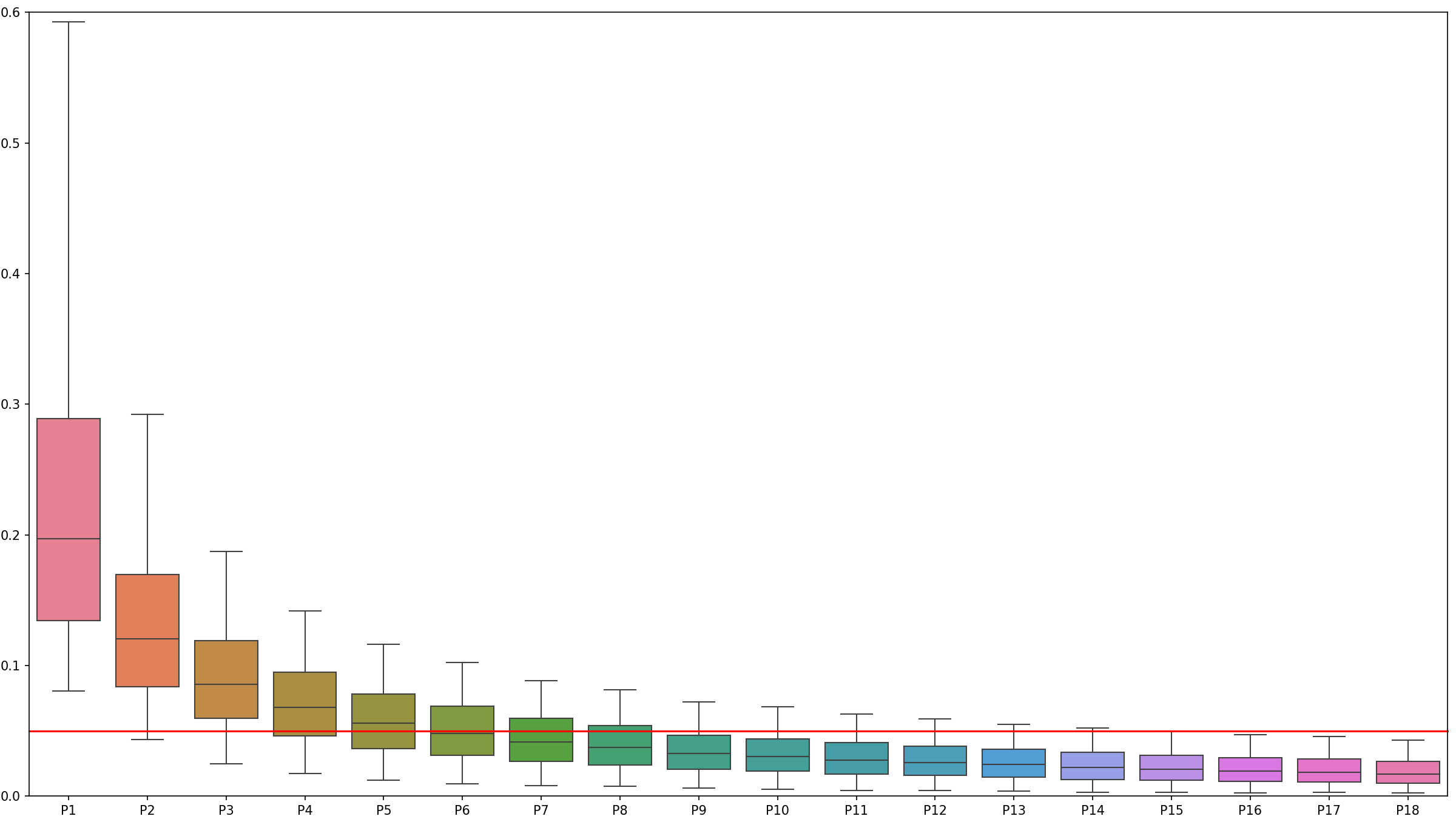
This shows the average ‘influence’ of each successively distant primary school on working out the ‘local area. FSM measure. The line in the middle of each box shows the median value. For example, the leftmost box means we can say that, on average the nearest single primary school accounts for about 0.2 or 1/5 of the measure.
The ‘whiskers’ have been set to show the 5th and 95th percentiles. The horizontal red line is at 5%. To meet the target the rightmost box including its upper ‘whisker’ must be wholly underneath the red line. This shows that for 95% of secondary schools the 18th nearest primary accounts for less than 5% of the weighting.
It takes some time to calculate all the results before they can be checked and enhancements to the initial algorithm (described below) meant increasing the number of primary schools checked. The final data and the plot above were both based on checking the 18 nearest primary schools to each of the 3000+ English secondary schools. The plot shows that the last three are fully below the red line so this number could have been reduced but there is no real benefit.
The results
Research by the Sutton Trust found, “80% of parents believe state schools should have a mix of pupils from different backgrounds. 76% say that intakes should reflect the make-up of the local community, and 69% say high achieving schools should make an effort to take in pupils from less well-off backgrounds.” (Cullinane 2020).
This method provides an objective quantifiable measure of whether a specific secondary school’s intake reflects its local community. Individual schools can be plotted on a graph like this.
Gap between Kent schools and their local communities. Open full screen.
This shows just the secondary schools in Kent (about 100 of them). Hovering over each point brings up the school its details. Those above and to the left of the line admit relatively more deprived pupils than the local community. Those to the bottom right admit fewer. The schools have also been categorised as either Comprehensive, Faith, or Selective. Clicking on the legend for each can remove and add them from the graph.
Other generalisations can be made by looking at all 3,070 secondary schools:
- 341 single sex schools on average admit 7.15% fewer disadvantaged children compared to the local area. The 2,729 mixed sex schools on average admit 0.75% more disadvantaged children.
- 163 selective (grammar) schools admit 17.4% fewer disadvantaged children. 533 faith schools admit 2.7% fewer disadvantaged children. The remaining 2,374 secular comprehensive schools admit 1.64% more disadvantaged children compared to their local area.
A closer look at faith schools
Although overall faith schools admit 2.7% fewer disadvantaged children, there is a lot of variation between different faiths. The following table breaks down all of the 533 schools which the DfE have recorded a ReligiousCharacter value against. These values don’t always make sense. For example there are 7 secondary schools categorised as Church of England/Roman Catholic. It seems almost as if whoever entered the data wasn’t too sure which of the two was correct so hedged their bets! No attempt has been made to rationalise the DfE’s categorisations, for example by adding the one “Anglican/Church of England” school to the other CoEs or visiting the websites of schools to check.
The following table shows ReligiousCharacter, Gap size and number of schools in each category. A “negative gap” indicates the schools admit more disadvantaged children compared to the local area. The rows can be sorted by clicking on the headings.
| ReligiousCharacter | Gap | #Schools |
|---|---|---|
| Roman Catholic | 4.09 | 289 |
| Church of England | 0.83 | 170 |
| Christian | 3.37 | 41 |
| Muslim | 5.59 | 18 |
| Jewish | 14.28 | 14 |
| Church of England/Roman Catholic | 0.70 | 7 |
| Roman Catholic/Church of England | -1.26 | 5 |
| Catholic | 4.87 | 3 |
| Sikh | 16.45 | 2 |
| Anglican/Church of England | -12.50 | 1 |
| Church of England/Christian | -1.10 | 1 |
| Greek Orthodox | -2.50 | 1 |
| Hindu | 10.20 | 1 |
Categorising ‘inclusivity’
As part of the requirements to make it easy to understand, the Fair Admissions Advisor presents a categorical interpretation of gap sizes in plain English. After calculating the gap for each school, the 10th, 25th, 75th and 90th percentiles were found. Schools were then classified into one of these five ordinal descriptive categories.
| Measure | Description |
|---|---|
| Below 10% quantile | very inclusive |
| Between 10% and 25% quantiles | more inclusive than most |
| Between 25% and 75% quantiles | broadly typical |
| Between 75% and 90% quantiles | less inclusive than most |
| Above 90% quantile. | among the least inclusive |
This plot shows the distribution of all 3,070 secondary schools’ ‘gaps’.
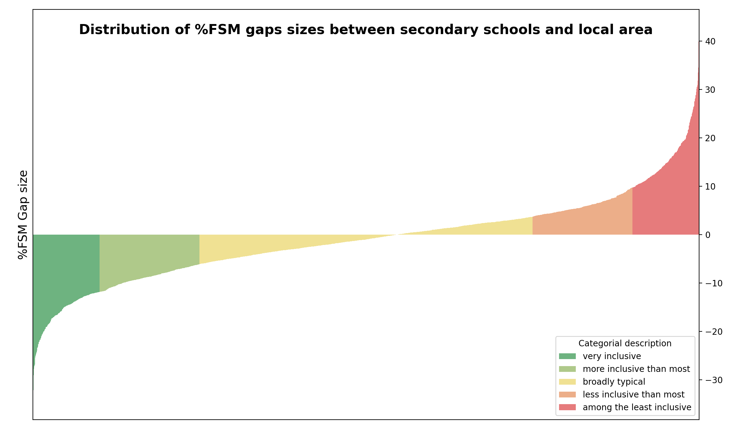
This shows at a glance that the ‘nearest primaries local FSM’ method doesn’t need much calibration ‘out of the box’. The proportion of FSM children in schools should match the proportion in the community. The median gap for all schools should be zero. This would mean the two yellow areas are equal in area. The uncalibrated median gap size is -1.03%. If the y-axis of the above plot was moved down by 1% the two halves of the plot would balance around zero. The final results are adjusted by this amount.
League tables!
This table shows the ten schools with the highest gaps between the proportion of disadvantaged children they admit and those attending local primary schools.
| School | School FSM | Local FSM | Gap |
|---|---|---|---|
| Birmingham Ormiston Academy | 13.7 | 57.4 | 43.7 |
| The Queen Elizabeth’s High School, Gainsborough | 8.7 | 49.6 | 40.9 |
| King Edward VI Five Ways School | 17.3 | 55.3 | 38 |
| St Anselm’s College | 11.4 | 46.9 | 35.5 |
| The Blue Coat CofE School | 11.8 | 46.4 | 34.6 |
| Skegness Grammar School | 22 | 56.3 | 34.3 |
| Dover Grammar School for Boys | 17.4 | 50.2 | 32.8 |
| King Edward VI Handsworth Grammar School for Boys | 14.3 | 46.2 | 31.9 |
| The North Halifax Grammar School | 5.1 | 36.8 | 31.7 |
| Beis Yaakov High School | 2 | 33.6 | 31.6 |
Improvements
This article was initially written in March 2025 to describe the basic approach of using local primary schools weighted by size over the square of their distance to work out the “local area FSM”. It has been updated a few times since to reflect enhancements to this method.
Income Deprivation Affecting Children Index (IDACI)
Before March had finished, the code had already been modified to compare schools against Income Deprivation Affecting Children Index (IDACI) Score using an inverse square weighting to distance.

This involves about a billion distance calculations and takes about three hours to run but has some advantages. IDACI is a direct measure of deprivation so offers a better method for education researchers. Because primary schools aren’t being used as the ‘yardstick’ their inclusivity can also be checked. These two plots compare the IDACI based measures against the ‘nearest primary’ method for secondary schools with different tuning parameters.
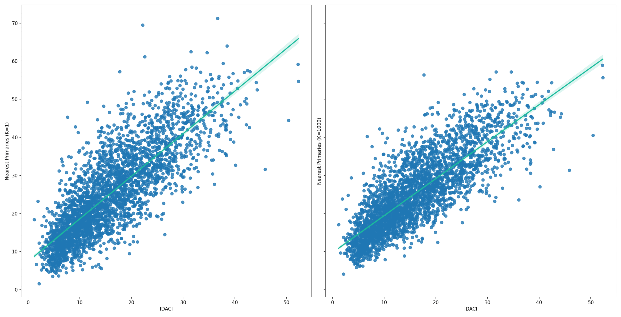
The plot on the left adds a fixed one metre to the calculated distances to nearest primary schools. The one on the right adds 1,000 metres (1km). The values here are closer to the trend line indicating a better match to the IDACI based measure of ‘local area’ disadvantage.
There was a lot of discussion over whether the Fair Admissions Advisor should use the IDACI method instead of nearby primary schools which in turn may not reflect their local community. Analysis of travelling distances showed that children tend not to travel very far to attend primary schools and the above plots show a good correlation between the two methods, especially if a fixed 1km is added to the distance to each primary school.
The big disadvantage of the IDACI method is it is a different measure of child poverty compared to FSM. The Fair Admissions Advisor needed to be easy for ordinary people to understand. The public are familiar with FSM. Not so IDACI. To extend the usual metaphor, it’s better to compare apples with apples especially if the alternative (IDACI) is a kumquat which hardly anyone has heard of.
A bit less local?
When the initial ‘local area FSM’ figures were calculated some odd results were noticed. This is not uncommon when making statistical generalisations. There are often specific examples that that don’t fit. In this case, testing revealed that Astor School’s ‘local FSM’ rate was 45.1% whilst neighbouring Dover Boys was 53.5%.
It doesn’t make sense for the ‘local FSM’ rates for two adjacent secondary schools to differ by so much, but equally it doesn’t make sense to have two adjacent secondary schools! Plotting the neighbouring secondaries (green) and the nearest four primaries (red) on a map helps understand how this particular example came up and suggest how the ‘local FSM’ formula could be improved.
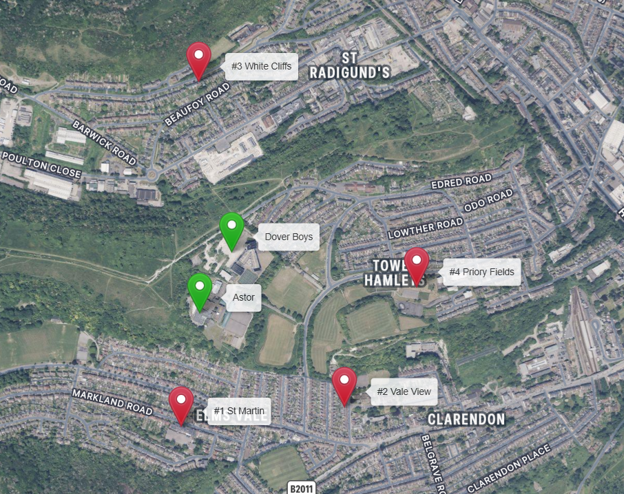
There are roughly five primary schools for each secondary school. If they were just located to serve populations we’d always expect to find some primaries between any pair of secondary schools. However, this is Kent where schools are located to serve segregation. Primary schools between the secondaries schools would normally provide a gradual transition between areas of different affluence but there are none between Astor and Dover Boys!
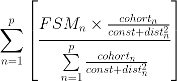
Another factor here is the rapid change in demographics over a very small area. St Martins has only 22.2% FSM whilst the other three have 50-60%. Because the formula uses straight line distance calculations it’s 50% further to Dover Boys. This would be less if a real world ‘by road’ distance was used but this is impractical. There are several very specific factors here that combine to create the unusual result. It would be wrong to change the model to address a specific set of circumstances, but this suggests that the initial model was a too ‘sensitive’ to relatively small changes in schools’ locations. The solution was to add a constant value  to the distance to each primary school:

This ‘spreads the net a bit wider’ so it became necessary to increase the number of primary schools checked. This is a good sign. It shows that the results are not based on too few primaries. As per the box plot above, the single nearest primary accounts for a fifth of the measure on average. Both the number of primaries checked (p) and the distance constant (k) are configurable parameters in the code. With  (1 kilometre) the difference in ‘local area’ FSM between these two schools drops to a very reasonable 1.5%.
How local should the local community be?
The Sutton Trust’s research concluded parents think schools’ admissions should reflect the ‘local community‘. However, local community is subjective. In this context it is based on how far children should travel to a school of choice. This becomes controversial because one parent’s desire that local community is broadly enough defined to enable them to apply to a particular popular school which has a finite number of spaces comes at the expense of another more local parent’s choice.
There is a minimum amount of effort involved in any journey to school even if the school is next door. It is not five times more effort to take the bus five stops than just one. For that reason, adding a fixed distance to each primary school makes logical sense. Where to set this is a matter of ideology. Thatcher’s 1980s neo liberalisation of state education provision created a parentocracy. In theory, parents are free to choose which schools they send their children to. In practice, this creates winners and losers and invariably those with the least social and economic capital end up losing.
Setting it to 1km reduced the difference in ‘local community’ FSM between Astor and Dover Boys to under 1.5%. That addresses the otherwise bizarre situation of having two schools next door with different ‘local area FSM’. It also reduced the weight given to just the nearest one primary from about 50% to 25% of the measure. Neoliberals would want to see this value increased. Those who consider local schools should be for local children would prefer it to be close to zero. The value is configurable. Just don’t expect agreement between these two opposing camps on where it should be set.
The Maths
The initial version of the ‘local area FSM‘ formula, as per the example based on just based on the three nearest primary schools, can be generalised for any number  primary schools and formally expressed as:
Adding a constant to the distance is a very minor modification to the equation:
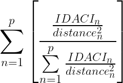
The IDACI formula is simpler. LSOAs are designed to contain similar population sizes so don’t need to be weighted.
Code and data used is available at https://github.com/jamescoombs3/heart.
For those just interested in the data created for the Fair Admissions Advisor, this can be downloaded as a CSV file here.
References
BBC News, Academies Bill ‘rushed through’ claim, [2010] https://www.bbc.co.uk/news/education-10664722
Department for Education, Get Information About Schools data download page.
Department for Education, A guide to the single academy model funding agreement, [2013]. gov.uk website (pdf)
Fitz, J., Taylor, C., & Gorard, S. (2002). Local education authorities and the regulation of educational markets: four case studies. Research Papers in Education, 17(2), 125-146. https://doi.org/10.1080/02671520210122900
Reed, W.J. (2002), On the Rank-Size Distribution for Human Settlements. Journal of Regional Science, 42: 1-17. https://doi.org/10.1111/1467-9787.00247
Office for National statistics, National Travel Survey, NTS0614: Trips to and from school by age, trip length and main mode, aged 5 to 16: England, 2002 onwards. Accessed via https://www.gov.uk/government/statistical-data-sets/nts06-age-gender-and-modal-breakdown#school-travel





Recent Comments