
YouGuv created this Sankey diagram to illustrate what effect Brexit would have on a second Scottish independence referendum.

It turns out, the answer was not a lot, but the choice of diagram is good for representing the interaction between different dimensions (in this example, historic voting and future intentions) within a given ‘population’.
Sankey diagrams consist of three key elements:
- Nodes: These are categorical values. A finite, ideally relatively low, number of options such as voting “yes”, “no” or “don’t know”.
- Dimensions: These are a collection of nodes. In this example, one dimension is how people voted in the past, the other is how they intend to vote in future.
- Pipes: These represent the number of people that belong in specific nodes for each dimension. For example those who voted Remain and Yes (yellow) but now intend to vote No (purple) are represented by the thin solid yellow line.
Sankeys are a bit like having multiple pie charts but throwing in the ability to see how many of those in a given slice of pie map to a completely different chart. Here we can see from the slenderness of the solid yellow line that not many people voted Remain/Yes but now intend to vote No. Conversely, fat pipes show a correlation between nodes between different dimensions. The prevalence of fat ‘pipes’ shows that the Scots haven’t really changed their minds that much.
Sankey and school stratification
I wanted to see how well Sankey diagrams could illustrate the different facets of secondary education within a local authority. Starting with datasets published by the DfE (Schools Pupils and Characteristics and the England KS4) I extracted data for the 20 secondary schools in Wirral to obtain the following dimensions:
- Socioeconomic status [FSM|non FSM] (FSM = Free School Meals)
- KS2 Prior attainment [low|medium|high]
- Sex [Boy|Girl|Coed]
- Admissions policy [Grammar|SecMod]
This post contains a selection of the good the bad and the downright ugly which can be derived from these data.
SES >> School
Producing Sankey plots is very labour intensive because each node and pipe needs to be individually defined with three or four parameters. This was my first working example, mapping the numbers of FSM children to each school.
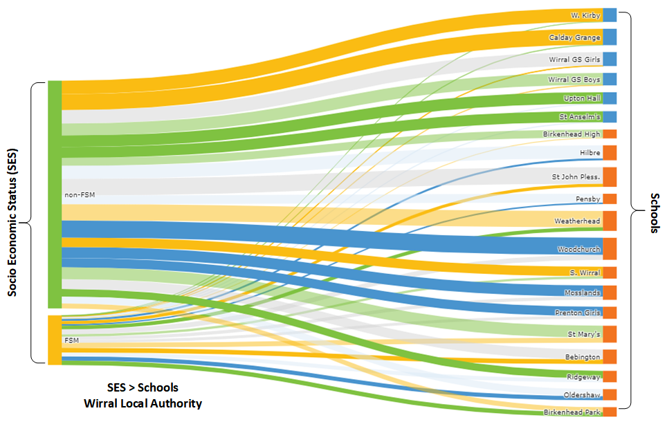
Plotly’s implementation of Sankey auto-arranges the nodes to minimise the amount of crossing over but as a consequence, all the grammar schools (blue) are at the top. This wasn’t intentional!
SES >> School >> sex
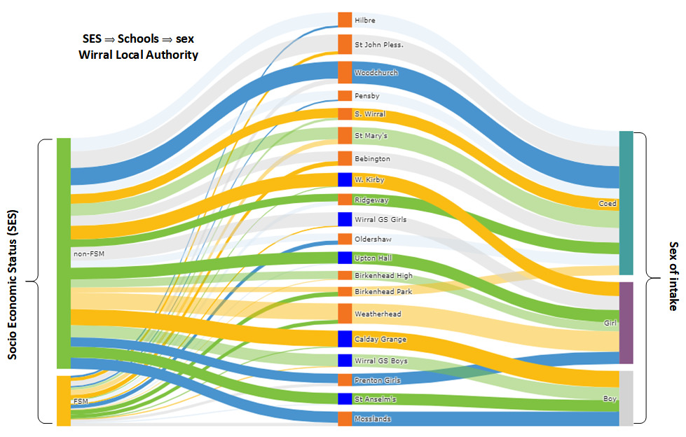
For the next plot, I added the sex of those admitted. This is a categorical variable describing the school’s admissions policy so each school leads to only one (sex) admissions policy type. This mixes up the schools which I prefer.
SES >> School >> PriorAttain
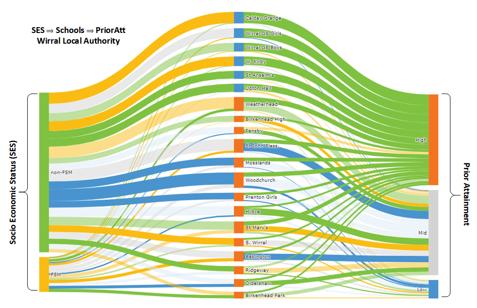
This time the rightmost dimension is prior attainment and once again plotly ends up sorting the schools by admissions policy!
Coloured flows
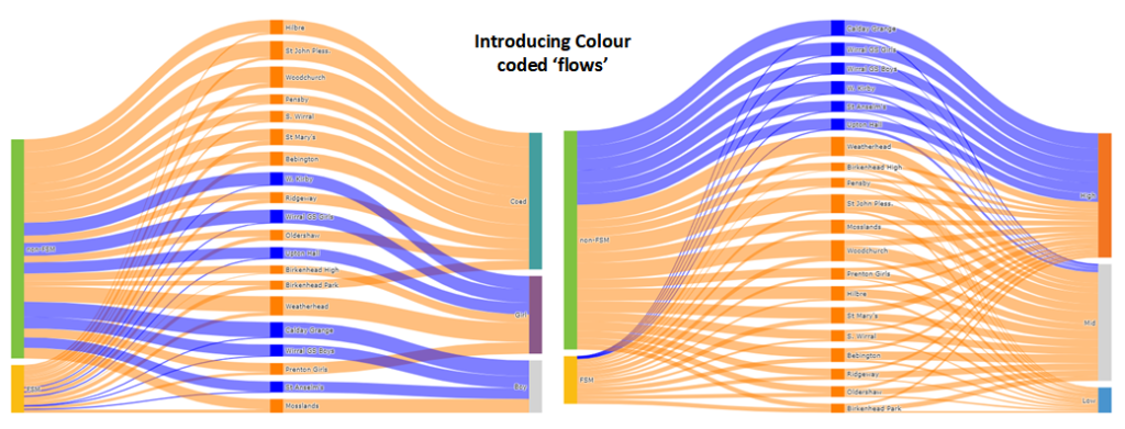
Because of the effort in manually specifying every element of the chart, up to this point the colours were all random. These two plots were a repeat of the previous two but with some colour coding of the ‘flows’. (Blue=grammar, Orange=SecMod)
Four dimensions!
My first attempt to get four dimensions (prior attainment, SES, School and sex) on a single graph.
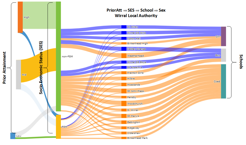
Well it’s interesting! It demonstrates a limitation with Plotly’s implementation of the Sankey graph. There are exacly 17,800 children in this cohort, regardless of how they’re divided. The widths of all the ‘flows’ add up to the same in each section. The nodes should also add up to the same height, but the non-FSM|FSM nodes are twice as high as they should be.
It’s as if Plotly treats the 17,800 children flowing from prior attainment (far left) to SES as a completely different cohort to the 17,800 children which flow from SES into the schools. There seems to be a maximum of three possible dimensions, although colour can add further information.
SES >> School >> [PriorAttain AND sex]
This plot covers the same values as the previous but here prior attainment are both on the right. It sort of works, but notice that for each school the ‘outflow’ on the right is double the size of the ‘inflow’ on the left.

Two in two out
One way to ‘fix’ is to add another dimension …
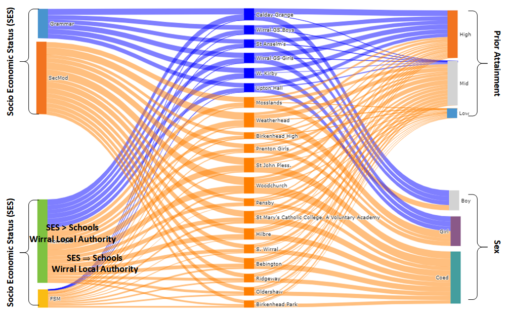
… but this groups the grammar schools together again!
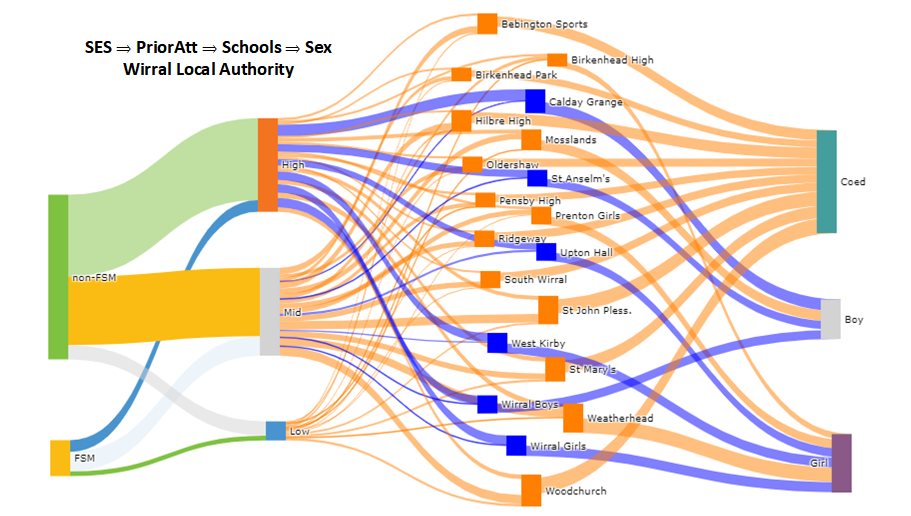
The ugly!!
As promised! Plotly allows the nodes to be dragged into different positions. This was another attempt to plot four dimensions on a graph and it really doesn’t look pretty!
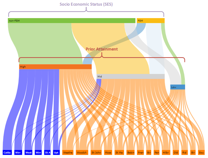
SES >> PriorAttain >> School
It’s also possible to rotate the ‘flow’ from top to bottom. This shows how children who start out disadvantaged perform lower at KS2 and in turn are less likely to get into the grammars. Some individuals will make it from the top right to bottom left but they’re the exception. These are the anecdotes trotted out to support the claim that grammar schools promote social mobility.
Sex AND [SES >> PriorAttain] >> School
The right hand side of this last plotis as per the above but single sex admissions are added as a second input on the left. As previously noted, a limitation of the Sankey is the schools are really double the width they should be, but this still provides a good understanding of how single sex entry and socioeconomic status (SES) interact in Wirral’s secondary schools.

One final idea is to change the sex category. Instead of categorising each school’s overall sex admissions policy as [Coed|girl|boy] capture the numbers of girls and boys at each school. The ‘sex’ dimension (top left) would contain just the two nodes boy or girl. Coed schools would have a pipe leading from each. Single sex schools would have just one.
This might highlight some of the issues that single-sex entry creates in terms of narrowing choice, however it neds a lot of restructuringt the data, so that’s one I’m leaving for a rainy day!
The code
The actual plotting of these diagrams only requires a few tens of lines of code. The hard bit is defining two data structures, one for the nodes, the other for the links. I found an effective way to do this was to use Excel’s concatenate function to write the code to set these variables then copy and paste into the program. The Excel spreadsheet and a Jupyter Notebook which does the actual plotting can both be found on GitHub.
Sankey Trivia
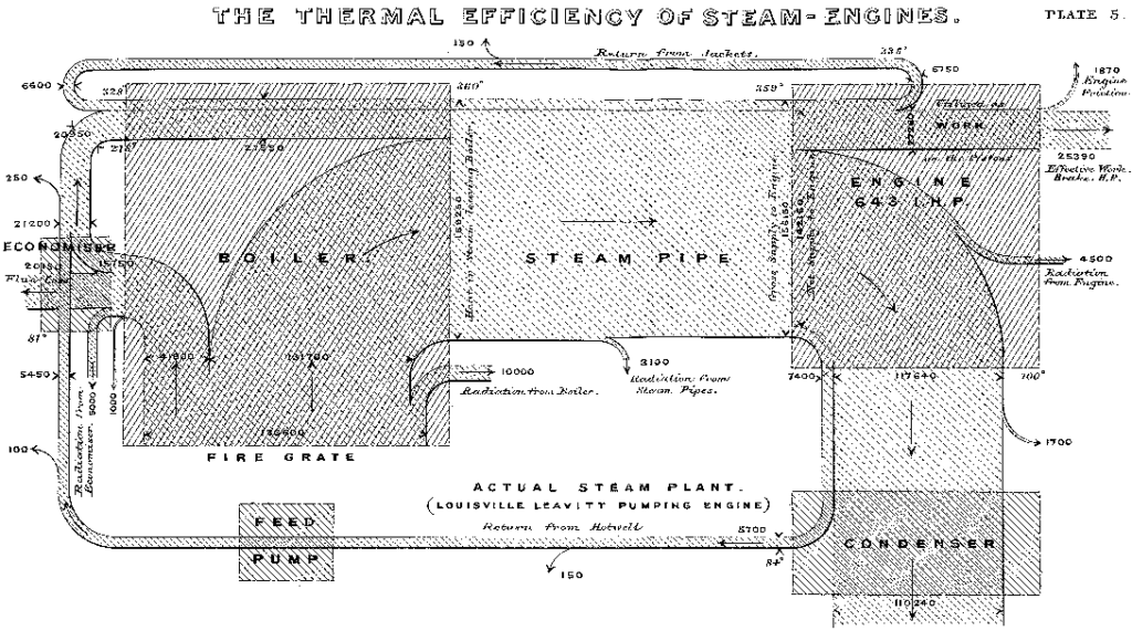
These ultra-modern looking diagrams are named after the Victorian industrialist Captain Matthew Henry Phineas Riall Sankey. In 1898 he created this map of energy losses in a system, representing the amount of energy by the width of the ‘pipes’.
Sankey gave his name to this type of chart, but he was very much building on the work of others. Half century earlier, in 1845, pioneer of statistical graphics Charles Minard plotted the traffic between Dijon and Mulhouse using the thickness of lines to represent volumes. Minard is best known for his 1869 Tableau Graphique of Napoleon’s march on Moscow.
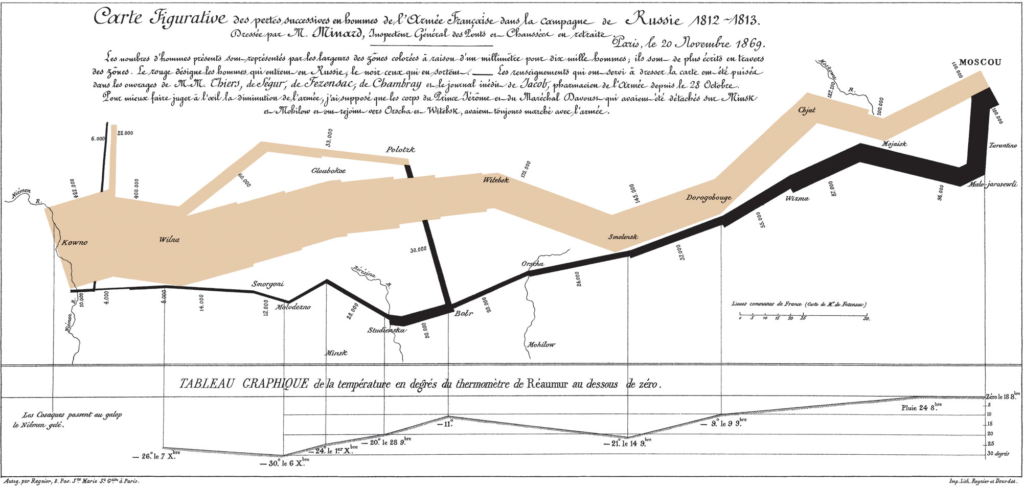
This graphically plots the demise of the 422,000 strong army that started out in 1812. Each millimetre represents 10,000 men; beige showing the advance and black the retreat. Less than a quarter made it to Moscow. Of those only 10,000 made it back to Poland.

Leave a Reply